Sumif Not Blank Can Be Fun For Everyone

There's an additional shortcut we can use right here: when utilizing the = indication, we don't need to include the "="& part of our condition. If Excel doesn't see any kind of logical drivers, it will certainly assume that we are trying to ensure that the worth in a certain cell amounts to what we have in our variety.

Now that you're comfy with SUMIF, you may be questioning whether it's possible to sum a variety based on numerous criteria instead of a solitary one. You remain in luck-- our SUMIFS tutorial will reveal you how!.?.!! Job smarter, not harder. Register for our 5-day mini-course to get must-learn lessons on obtaining Excel to do your benefit you.

Why to rethink the method you do VLOOKUPs ... Plus, we'll expose why you shouldn't make use of Pivot Tables and what to use instead ... Please enable Java Manuscript to see comments.

The SUMIF and SUMIFS feature in Microsoft Excel is an easy, yet powerful calculation device. This tutorial will certainly reveal you just how this feature works, as well as supply examples of how to utilize it. A lot of you know that the AMOUNT function computes the overall of a cell range.

The Definitive Guide for Sumif Multiple Criteria

It states, "Only AMOUNT the numbers in this array IF a cell in this range consists of a particular value." Appropriate phrase structure: =SUMIF(array, standards, sum_range) Variety and requirements are important parts of any kind of SUMIF equation; while the sum variety is optional. What does each part do, in English? Range - The series of cells you desire Excel to browse.

Requirements - Defines the flag Excel is to make use of to figure out which cells to include. Utilizing our spread sheet instance below, the requirements can be "Non Edible", "October" or "Vehicle", to call a few. Oftentimes, it's just a number. Maybe higher than, less than, or equivalent to, as well.

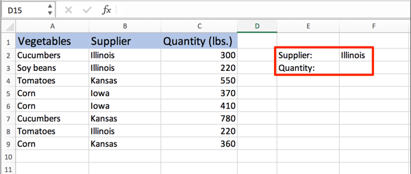
Specifies the cells to amount. This array holds the real numbers. If it's omitted of the formula, the feature amounts the variety. As with range, this could be a block of cells, column or rows. For this tutorial, we're mosting likely to make use of a simple table to track house expenditures for 2 months.

In this example, our objectives are: determine monthly home prices provide a failure of total prices automatically update of calculations Let's start! (1) Spreadsheet Arrangement Create a table called COST TABLE with the following headings: Month, Kind, Sub-type, and Expense. Load them in, as displayed in the screenshot listed below: Develop a table called COMPUTATIONS, and also include the adhering to headings in the initial column: October, Food, Non Edible, November, Food, Non Edible, and Complete - following the layout listed below: (2) Create the SUMIF Function in the COMPUTATIONS table The SUMIF function in C 4 (column C is the Total amounts column) totals the Expense column depending on the Kind of the entry.

3 Easy Facts About Sumif Multiple Criteria Shown

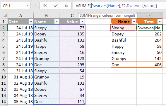
If intended to complete food for November as well, I 'd utilize the variety G 4: G 13. Currently, if the Month column was not arranged, after that I would certainly need to use the SUMIFS function and also specify to criteria - e.g., =SUMIFS(I 4: I 13, F 4: F 13,"October", G 4: G 13,"Food") This generates the exact same results - $4.24.

_ Correct syntax: _ =SUMIFS(sum_range, criteria_range 1, requirements 1, criteria_range 2, standards 2, criteria_range 3, requirements 3 ...) (3) ** ** Automatic Updates In order for the calculation table to upgrade when a number is transformed or when a brand-new row is included, you require to change the EXPENSE TABLE from a variety to an actual table.

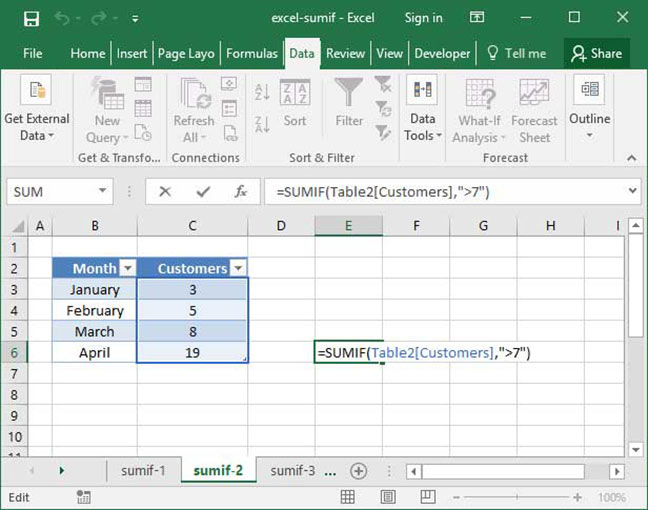
Ensure you do not include the COST TABLE tag in your range selection: Now, you'll need to rewrite your functions. As an example, cell C 4 will now be - =SUMIF(Table 1 [Month],"October", Table 1 [Cost] See the distinction? Rather of the variety, there is the table name as well as header. Update all of the functions to match this syntax: Now when you make any changes the ESTIMATIONS table will certainly update instantly (contrast both Overalls columns to see the modifications).

( 4) Much more Examples SUMIF can utilize requirements such as better than or much less than. As an example, if you only desire to complete costs larger than $4, you can create: Instance 1: =SUMIF(I 3: I 12,"> 4", I 3: I 12) SUMIF features can be created without the amount range if it's the exact same as the array.

Getting My How To Use Sumif To Work

If the criteria is an expression or text, structure it in quotes. Example 3: without quotes, if the variety equates to the worth in cell I 3: =SUMIF(I 3: I 12, I 3) Integrate SUMIF with other features for higher computations, such as summing and after that separating, by putting the whole function in parenthesis: Instance 4: =SUM (( SUMIF (I 3: I 12,"> 4"))/ 3) Suggestion: Keep in mind that Excel determines using the basic order of procedures.

By including specifying columns instead of using spreadsheets (a Month column rather than splitting October costs and also November sets you back into separate sheets, for instance), you maintain all the data on a solitary sheet. Consequently, it comes to be simpler to sort, compare, and also modify groups. Currently, when you include in your Cost Table, your computations will automatically upgrade.

SUMIF with OR (Tabulation) SUMIF with OR in Excel Exactly How to Utilize SUMIF with OR in Excel? SUMIF is among the functions which is quite beneficial to find the overalls of similar values. It lowers the time when we are working with a big amount of information as well as need to compute the sum of worths of comparable nature data.

SUMIF feature will carry out SUM(addition) when the IF condition satisfies. It is really simple to use. Start Your Free Excel Program Excel functions, formula, charts, formatting creating excel dashboard & others Syntax of the SUMIF function Variety-- A series of cells on which the requirements or problem is to be applied.

sumif excel less than today excel sumif nasıl kullanılır excel sumif date