4 Easy Facts About Excel Shortcuts Described

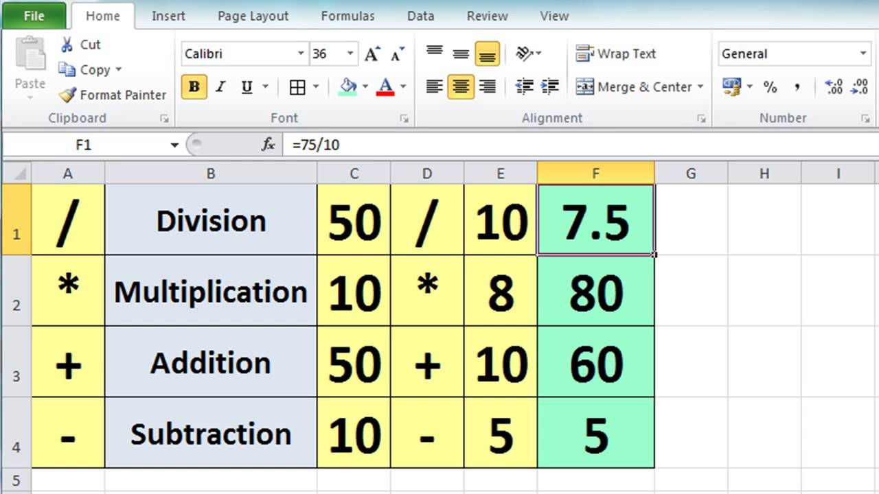
By pushing ctrl+shift+facility, this will determine and return worth from numerous ranges, instead of simply individual cells added to or increased by one an additional. Computing the sum, product, or ratio of individual cells is simple-- just utilize the =SUM formula and also get in the cells, worths, or range of cells you wish to execute that math on.

If you're looking to discover total sales profits from numerous sold devices, for example, the selection formula in Excel is best for you. Below's how you would certainly do it: To start making use of the selection formula, type "=AMOUNT," and in parentheses, enter the very first of 2 (or three, or 4) varieties of cells you wish to increase together.

This means reproduction. Following this asterisk, enter your second range of cells. You'll be multiplying this 2nd series of cells by the very first. Your progression in this formula should now appear like this: =SUM(C 2: C 5 * D 2:D 5) Ready to press Go into? Not so quickly ... Due to the fact that this formula is so challenging, Excel gets a various keyboard command for selections.

This will certainly recognize your formula as a selection, wrapping your formula in brace personalities and successfully returning your item of both ranges incorporated. In profits computations, this can lower your effort and time considerably. See the final formula in the screenshot above. The MATTER formula in Excel is denoted =MATTER(Beginning Cell: End Cell).

For instance, if there are 8 cells with gone into worths between A 1 as well as A 10, =COUNT(A 1: A 10) will return a worth of 8. The MATTER formula in Excel is especially valuable for large spread sheets, where you desire to see the amount of cells contain real entries. Don't be fooled: This formula won't do any kind of math on the values of the cells themselves.

Some Known Details About Excel Jobs

Using the formula in strong over, you can easily run a matter of active cells in your spread sheet. The result will look a something similar to this: To execute the typical formula in Excel, get in the worths, cells, or variety of cells of which you're calculating the standard in the layout, =AVERAGE(number 1, number 2, etc.) or =STANDARD(Beginning Value: End Worth).

Finding the standard of a variety of cells in Excel keeps you from having to discover individual amounts and afterwards doing a separate division formula on your total. Using =AVERAGE as your initial text access, you can let Excel do all the work for you. For reference, the average of a team of numbers is equal to the amount of those numbers, divided by the number of items in that group.

This will return the sum of the worths within a preferred variety of cells that all meet one criterion. For instance, =SUMIF(C 3: C 12,"> 70,000") would certainly return the amount of worths in between cells C 3 as well as C 12 from just the cells that are above 70,000. Allow's say you wish to establish the profit you created from a listing of leads who are connected with details location codes, or calculate the amount of specific staff members' incomes-- yet only if they fall above a certain amount.

With the SUMIF function, it does not need to be-- you can quickly add up the amount of cells that satisfy certain requirements, like in the income instance over. The formula: =SUMIF(range, requirements, [sum_range] Range: The range that is being tested using your criteria. Standards: The standards that establish which cells in Criteria_range 1 will be combined [Sum_range]: An optional series of cells you're mosting likely to add up along with the initial Range entered.

In the example listed below, we wanted to determine the amount of the salaries that were above $70,000. The SUMIF function built up the buck quantities that went beyond that number in the cells C 3 with C 12, with the formula =SUMIF(C 3: C 12,"> 70,000"). The TRIM formula in Excel is represented =TRIM(text).

Indicators on Excel Skills You Should Know

As an example, if A 2 consists of the name" Steve Peterson" with undesirable areas before the given name, =TRIM(A 2) would certainly return "Steve Peterson" with no rooms in a new cell. Email and submit sharing are terrific tools in today's work environment. That is, till one of your colleagues sends you a worksheet with some truly fashionable spacing.

Instead of painstakingly getting rid of as well as adding spaces as needed, you can tidy up any irregular spacing utilizing the TRIM function, which is made use of to remove extra rooms from data (with the exception of single rooms in between words). The formula: =TRIM(message). Text: The message or cell from which you intend to remove spaces.

To do so, we entered =TRIM("A 2") into the Solution Bar, and also reproduced this for every name listed below it in a new column alongside the column with unwanted rooms. Below are some other Excel solutions you could locate valuable as your information administration requires expand. Allow's say you have a line of message within a cell that you wish to damage down right into a few different sectors.

Function: Used to remove the first X numbers or personalities in a cell. The formula: =LEFT(text, number_of_characters) Text: The string that you wish to draw out from. Number_of_characters: The number of personalities that you want to extract beginning with the left-most character. In the instance below, we got in =LEFT(A 2,4) into cell B 2, and duplicated it right into B 3: B 6.

Purpose: Utilized to remove personalities or numbers between based upon position. The formula: =MID(text, start_position, number_of_characters) Text: The string that you desire to extract from. Start_position: The setting in the string that you intend to start removing from. For instance, the very first position in the string is 1.

The Ultimate Guide To Excel If Formula

In this instance, we went into =MID(A 2,5,2) into cell B 2, and also duplicated it right into B 3: B 6. That permitted us to draw out both numbers beginning in the 5th position of the code. Function: Used to draw out the last X numbers or personalities in a cell. The formula: =RIGHT(text, number_of_characters) Text: The string that you want to draw out from.

formula excel gantt chart excel formulas by color formula excel greater than or equal to